How To Draw Nyquist Plot In Matlab Not Using Nyquist Command

Introduction to Nyquist Matlab

In this article, nosotros will larn how to create a Nyquist plot in MATLAB. Nyquist plots find their utility in analyzing system properties, like phase margin, proceeds margin & stability. As we volition motion forward in the article, nosotros will acquire how to create uncomplicated Nyquist plots and too Nyquist plots with complex atmospheric condition.

Understanding of Nyquist Plot

Nyquist plots also known as Nyquist Diagrams are used in signal processing and control engineering for plotting frequencies. Nyquist diagrams are used commonly to assess the stability of systems and besides to go feedback. Cartesian coordinates are used for Nyquist plots. On X-axis, we plot the real part of our transfer function and on Y-axis, we plot the imaginary part. To get a frequency plot, it is passed as a parameter and this results in a graph based on the frequency. Polar coordinates tin also be used for Nyquist plots. Here, radical coordinates are used to represent the transfer function's gain, and the corresponding angular coordinate is represented by the transfer role'southward phase.

Syntax for Creating a Nyquist Plot in Matlab

nyquist(sys)

Nyquist  part in MATLAB helps us in creating a Nyquist plot, related to frequency response produced past a dynamic model.

Let usa empathise this clearly with the assist of a few examples:

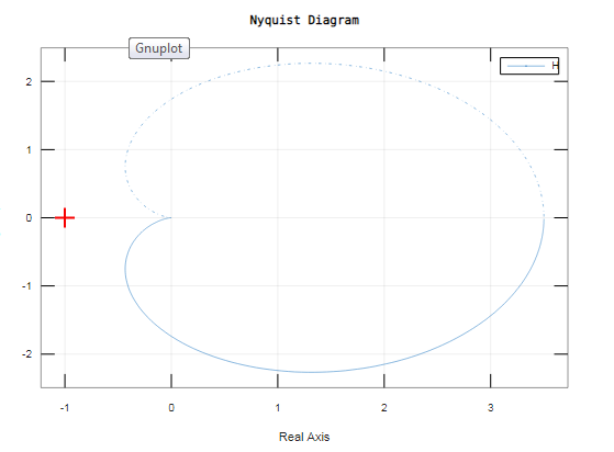
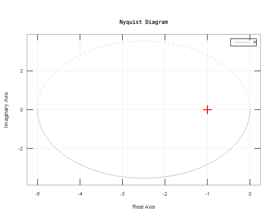
To draw a Nyquist plot, nosotros will first create a transfer function as follows:

H = 70 / (s+v) (s+ 4)

Now, this is a simple example without any other condition.

Nosotros tin write in a higher place system as:

H = 70 / (southward^2 + 9s + 20)

This transfer function is and so passed as an statement to our function 'nyquist'
i.enyquist(H)

This is how our input and output volition look like in MATLAB console:

Input:

H=tf([0 0 lxx],[1 9 20]); nyquist(H)

Output:

In the adjacent example, we will encounter a Nyquist plot with a pole at the middle/origin.

Hither is our transfer function:

H = 40 / s^3 + 2s ^ 2 + 3s + iv

This transfer part is then passed as an argument to our function 'nyquist'
i.enyquist(H)

This is how our input and output volition expect similar in MATLAB console:

Input:

H=tf([40],[three 2 3 4]); nyquist(H)

Output:

The system represented past our transfer function is having a pole located at the origin. This signifies the requirement of the detour effectually this pole. This is non shown on the plot created past Matlab.  In a arrangement like this where a detour is required around the pole, nosotros must sympathise the result of the detour.  In our case, since nosotros accept a single-pole located at origin & the detour has its radius approaching '0'&moving in the counter-clockwise direction, we translate that the missing part of the plot that MATLAB does not show is a semicircle. This semicircle lies at infinity and in the clockwise direction.

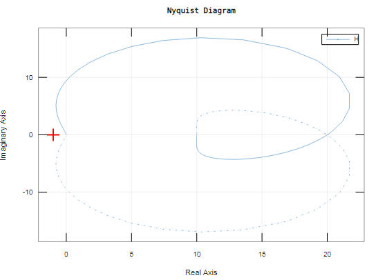
Let's take some other example with a different status:

In this example, we will see a Nyquist plot with a double pole at the center/origin.

Here is our transfer function:

H = 5s + 20 / s^3 + 5s^two

This transfer function is and then passed equally an argument to our function 'nyquist'
i.enyquist(H)

This is how our input and output will look like in MATLAB console:

Input:

H=tf([5 xx],[i five 0 0]); nyquist(H)

Output:

As nosotros can see from the plot obtained, the 2 branches are going off towards infinity.  Also, equally nosotros have a double pole at the origin, it tin be inferred that a counter-clockwise detour of 180° effectually the origin is yielding a clock-wise detour of 360°.

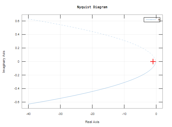
Finally, allow'due south take an example where transfer role will take i pole in RHP and the pole volition exist stable:

Here is our transfer function:

H = 20s + twoscore / s^two - 8

This transfer office is so passed every bit an argument to our role 'nyquist'
i.enyquist(H)

This is how our input and output will look like in MATLAB console:

Input:

H=tf([20 40],[ 1 0 -8]); nyquist(H)

Output:

So, in this article, we learned how to create a Nyquist plot in MATLAB. We can create both stable and unstable plots in MATLAB. As an boosted tip, please continue in heed that to brandish the real & imaginary part of our given frequency, we tin can activate the data markers in MATLAB. For this, we just demand to click at whatever point on the bend.

Recommended Manufactures

This is a guide to Nyquist Matlab. Hither nosotros hash out the Understanding of Nyquist Plot along with the Syntax for Creating information technology in Matlab. You may also take a look at the following articles to learn more –

Break in MATLAB
Summation in Matlab
Gaussian Fit Matlab
Matlab Errorbar